Machine Learning for Beginners: An Introduction to Neural Networks

博客（victorzhou.com/blog/intro-…）

1.Building Blocks: Neurons

神经网络的基本单位，神经元。 神经元接受输入，对其做一些数据操作，然后产生输出。 例如，这是一个2-输入神经元：

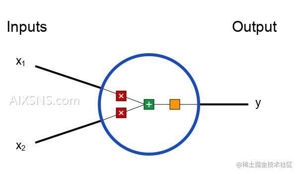
这里发生了三个事情。首先，每个输入都跟一个权重相乘（红色）：

x1→x1∗w1
x2→x2∗w2
然后，加权后的输入求和，加上一个偏差b（绿色）：

(x1∗w1)+(x2∗w2)+b
最后，这个结果传递给一个激活函数f：

y=f(x1∗w1+x2∗w2+b)
激活函数的用途是将一个无边界的输入，转变成一个可预测的形式。常用的激活函数就就是S型函数：

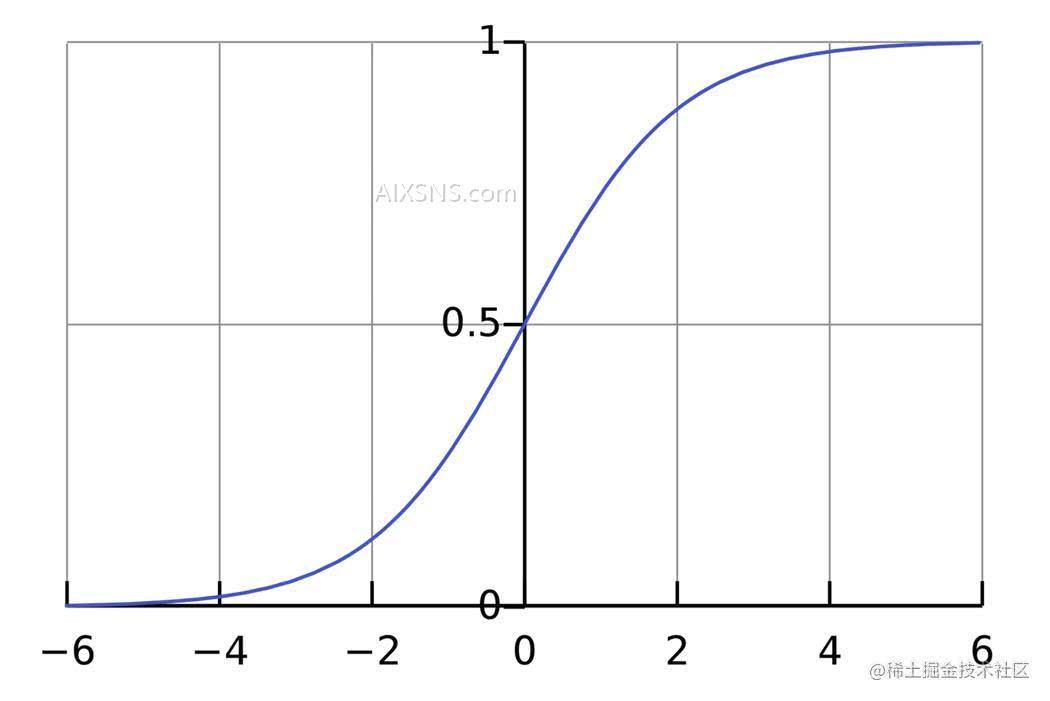
S型函数的值域是(0, 1)。简单来说，就是把(−∞, +∞)压缩到(0, 1) ，很大的负数约等于0，很大的正数约等于1。

假设：有一个神经元，激活函数就是S型函数，其参数如下：

（以向量的形式表示。现在，我们给这个神经元一个输入。我们用点积来表示：）当输入是[2, 3]时，这个神经元的输出是0.999。给定输入，得到输出的过程被称为前馈（feedforward）。

Coding a Neuron

Time to implement a neuron! We’ll use NumPy, a popular and powerful computing library for Python, to help us do math:

import numpy as np
# 编码一个神经元
def sigmoid(x):
    # 我们的激活函数: f(x) = 1 / (1 + e^(-x))
    return 1 / (1 + np.exp(-x))
class Neuron:
    def __init__(self, weights, bias):
        self.weights = weights
        self.bias = bias

    def feedforward(self, inputs):
        # 加权输入，加入偏置，然后使用激活函数
        total = np.dot(self.weights, inputs) + self.bias
        return sigmoid(total)


weights = np.array([0, 1])  # w1=0,w2=1
bias = 4  # b=4
n = Neuron(weights, bias)

x = np.array([2, 3])
print("feedforward")
print(n.feedforward(x))#0.9990889488055994

还记得这个数字吗？就是我们前面算出来的例子中的0.999。

2. Combining Neurons into a Neural Network

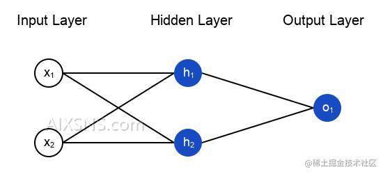
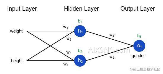
所谓的神经网络就是一堆神经元。这就是一个简单的神经网络：

这个网络有两个输入，一个有两个神经元（h1和h2）的隐藏层，以及一个有一个神经元（o1）的输出层。

An Example:Feedforward

我们继续用前面图中的网络，假设每个神经元的权重都是相同的，截距项也相同（），激活函数也都是S型函数。（all neurons have the same weights w=[0,1], the same bias b=0, and the same sigmoid activation function）Let 1h1,h2,o1 denote the outputs of the neurons they represent.

What happens if we pass in the input x=[2,3]?

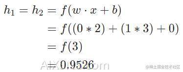
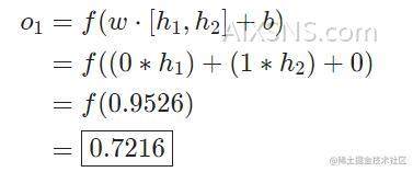
The output of the neural network for input x=[2,3] is 0.72160.7216. Pretty simple, right?

Coding a Neural Network: Feedforward

Let’s implement feedforward for our neural network.Here’s the image of the network again for reference:

import numpy as np
import jittor as jt
from sigmoid import Neuron



# ... code from previous section here
class OurNeuraIetwork:
    """
    A neural network with:
    - 2 inputs
    - a hidden layer with 2 neurons (h1, h2)
    - an output layer with 1 neuron (o1)
    Each neuron has the same weights and bias:
    - w = [0, 1]
    - b = 0"""


    def __init__(self):
        weights = np.array([0, 1])
        bias = 0
        # 这里是来自前一节的神经元类
        self.h1 = Neuron(weights, bias)
        self.h2 = Neuron(weights, bias)
        self.O1 = Neuron(weights, bias)


    def feedforward(self, x):
        out_h1 = self.h1.feedforward(x)
        out_h2 = self.h2.feedforward(x)
        # o1的输入是h1和h2的输出
        out_o1 = self.O1.feedforward(np.array([out_h1, out_h2]))
        return out_o1



network = OurNeuraIetwork()
x = np.array([2, 3])
print("network")
print(network.feedforward(x))  # 0.7216325609518421

We got 0.72160.7216 again! Looks like it works.

3.Training a Neural Network, Part 1

Say we have the following measurements:

Name	Weight (lb)	Height (in)	Gender
Alice	133	65	F
Bob	160	72	M
Charlie	152	70	M
Diana	120	60	F

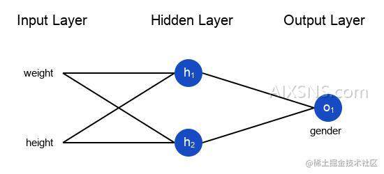
接下来我们用这个数据来训练神经网络的权重和截距项，从而可以根据身高体重预测性别:

我这里是随意选取了135和66来标准化数据，通常会使用平均值

We’ll represent Male with a 00 and Female with a 11, and we’ll also shift the data to make it easier to use:

Name	Weight (minus 135)	Height (minus 66)	Gender
Alice	-2	-1	1
Bob	25	6	0
Charlie	17	4	0
Diana	-15	-6	1

损失函数（Loss）

Before we train our network, we first need a way to quantify how “good” it’s doing so that it can try to do “better”. That’s what the loss is.

We’ll use the mean squared error (MSE) loss:

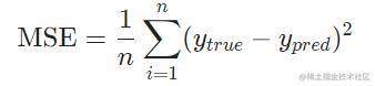
Let’s break this down:

• n is the number of samples, which is 44 (Alice, Bob, Charlie, Diana).
• y represents the variable being predicted, which is Gender.
• ytrue is the true value of the variable (the “correct answer”). For example, ytrue for Alice would be 11 (Female).
• ypred is the predicted value of the variable. It’s whatever our network outputs.

(ytrue−ypred)2 is known as the squared error. Our loss function is simply taking the average over all squared errors (hence the name mean squared error). The better our predictions are, the lower our loss will be!

Better predictions = Lower loss.更好的预测 = 更少的损失！

Training a network = trying to minimize its loss. 训练网络 = 最小化它的损失。

An Example Loss Calculation ：

Let’s say our network always outputs 0 – in other words, it’s confident all humans are Male . What would our loss be?

Name	ytrue	ypred	(ytrue−ypred)2
Alice	1	0	1
Bob	0	0	0
Charlie	0	0	0
Diana	1	0	1

MSE=1/4（1+0+0+1）= 0.5

Code:MSE Loss

Here’s some code to calculate loss for us:

代码：

# MSE Loss
import numpy as np



def mse_loss(y_true, y_pred):
    # y_true and y_pred are numpy arrays of the same length
    return ((y_true - y_pred) ** 2).mean()



y_true = np.array([1, 0, 0, 1])
y_pred = np.array([0, 0, 0, 0])


print(mse_loss(y_true, y_pred))  # 0.5

Nice. Onwards!

4.Training a Neural Network, Part 2

Example:Calculating the Partial Derivative

为了简化问题，假设我们的数据集中只有Alice :

Name	Weight (minus 135)	Height (minus 66)	Gender
Alice	-2	-1

Let’s initialize all the weights to 11 and all the biases to 00. If we do a feedforward pass through the network, we get:(把所有的权重和截距项都分别初始化为1和0。在网络中做前馈计算)

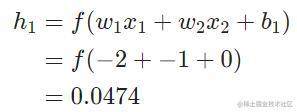
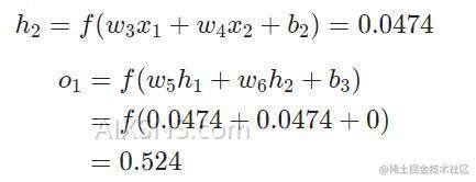
网络的输出是ypred=0.524，对于Male(0)或者Female(1)都没有太强的倾向性.Let’s calculate ∂L/∂w:

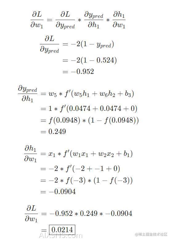
Reminder: we derived f′(x)=f(x)∗(1−f(x)) for our sigmoid activation function earlier.

**

Training: Stochastic Gradient Descent

现在训练神经网络已经万事俱备了！我们会使用名为随机梯度下降法的优化算法来优化网络的权重和截距项，实现损失的最小化.It’s basically just this update equation:

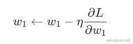
η is a constant called the learning rate that controls how fast we train.我们要做的就是用 w1减去η** ∂L∂w1.*

• If ∂L/ ∂w1 is positive, w1 will decrease, which makes L decrease.
• If ∂L/ ∂w1 is negative, w1 will increase, which makes L increase.

如果我们对网络中的每个权重和截距项都这样进行优化，损失就会不断下降，网络性能会不断上升。

我们的训练过程是这样的:

1. 从我们的数据集中选择一个样本，用随机梯度下降法进行优化——每次我们都只针对一个样本进行优化；
2. 计算每个权重或截距项对损失的偏导（例如∂L/ ∂w1等)；
3. 用更新等式更新每个权重和截距项；
4. 重复第一步；

Code: A Complete Neural Network

It’s finally time to implement a complete neural network:

Name	Weight (minus 135)	Height (minus 66)	Gender
Alice	-2	-1	1
Bob	25	6	0
Charlie	17	4	0
Diana	-15	-6	1

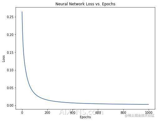
Our loss steadily decreases as the network learns:

搞定了一个简单的神经网络，快速回顾一下：

• 介绍了神经网络的基本结构——神经元；
• 在神经元中使用S型激活函数；
• 神经网络就是连接在一起的神经元；
• 构建了一个数据集，输入（或特征）是体重和身高，输出（或标签）是性别；
• 学习了损失函数和均方差损失；
• 训练网络就是最小化其损失；
• 用反向传播方法计算偏导；
• 用随机梯度下降法训练网络；