引言
在上一篇文章LightGBM中的CUDA算子(一)中我们介绍了LightGBM源码的结构和两种基础的cuda算子:并行规约、双调排序。这两类基础算子在LightGBM的boosting过程中用于直方图运算、增益计算、寻找分裂点等环节。接下来我们继续介绍LightGBM boosting过程中的一类cuda算子:直方图算子。
直方图算子
LightGBM直方图算子的定义与实现分别位于src/treelearner/cuda/cuda_histogram_constructor.h和cuda_histogram_constructor.cu中,包括直方图的构建、直方图运算两类,其中直方图构建算子有分别针对不同case的实现,如:不同特征类型(dense or sparse),不同的内存(global or shared)。下面我们以其中的一个case实现为例,介绍直方图构建。
直方图建构
CUDAConstructHistogramDenseKernel_GlobalMemory()算子展示了使用global memory对dense特征构造直方图的方法。首先我们要理清几个维度的概念:
n_data:数据量或样本量;
n_column: 字段数量或特征数量;
n_partition: 对特征进行分区得到的分区数量;
n_column_per_partition: 每个分区下分到的最多特征数量,如果不能整除,最后一个partition下分到特征数少于n_column_per_partition;
n_bin: 单个特征在构造直方图时所分的段数;
n_data_hat: 划归到叶子节点样本集的数量
// cuda_histogram_constructor.cu
template <typename BIN_TYPE>
__global__ void CUDAConstructHistogramDenseKernel_GlobalMemory(
        const CUDALeafSplitsStruct* smaller_leaf_splits, //封装了叶子节点分裂信息的结构体
        const score_t* cuda_gradients, //n_data
        const score_t* cuda_hessians, //n_data
        const BIN_TYPE* data, //n_data * n_column, 存放bin的编号
        const uint32_t* column_hist_offsets, //n_column
        const uint32_t* column_hist_offsets_full, // n_partition+1
        const int* feature_partition_column_index_offsets, // n_partition+1
        const data_size_t num_data, // n_data
        float* global_hist_buffer) // GridDim.x * n_partition * n_column_per_partition * n_Bin
{
    const int dim_y = static_cast<int>(gridDim.y * blockDim.y);
    const data_size_t num_data_in_smaller_leaf = smaller_leaf_splits->num_data_in_leaf; // 叶子节点分到的数据量n_data_hat <= n_data
    const data_size_t num_data_per_thread = (num_data_in_smaller_leaf + dim_y - 1) / dim_y; // 每个线程要处理数据量
    const data_size_t* data_indices_ref = smaller_leaf_splits->data_indices_in_leaf; // 叶子节点样本集数据索引
    const unsigned int num_threads_per_block = blockDim.x * blockDim.y;

    // 在n_column维度下分了多个partition, 每个partition下feature数量 n_column_per_partion = n_column/n_partition
    // 单个block负责单个partition, n_partition = n_block
    const int partition_column_start = feature_partition_column_index_offsets[blockIdx.x];
    const int partition_column_end = feature_partition_column_index_offsets[blockIdx.x + 1];
    // 该block对应data的起始位置
    const BIN_TYPE* data_ptr = data + static_cast<size_t>(partition_column_start) * num_data;
    // block下负责partition下的columns数量
    const int num_columns_in_partition = partition_column_end - partition_column_start;

    // block所负责partition在global_hist_buffer中地址偏移
    // 每个block在x维度上负责数据长度为n_column_per_partition*n_bin
    const uint32_t partition_hist_start = column_hist_offsets_full[blockIdx.x];
    const uint32_t partition_hist_end = column_hist_offsets_full[blockIdx.x + 1];

    // 2个位置分别用来放grad和hess
    const uint32_t num_items_in_partition = (partition_hist_end - partition_hist_start) << 1;
    const unsigned int thread_idx = threadIdx.x + threadIdx.y * blockDim.x;
    // n_column * n_bin
    const int num_total_bin = column_hist_offsets_full[gridDim.x];

    // global_hist_buffer数据采用scatter二维错位布局, shared_hist对应当前partition起始位置
    float* shared_hist = global_hist_buffer + (blockIdx.y * num_total_bin + partition_hist_start) * 2;

    // 循环兼容num_items_in_partition > block中线程数量场景,有个线程要处理多个地址
    for (unsigned int i = thread_idx; i < num_items_in_partition; i += num_threads_per_block) {
        shared_hist[i] = 0.0f; // 将global_hist_buffer初始化为 0
    }
    __syncthreads();

    const unsigned int threadIdx_y = threadIdx.y;
    const unsigned int blockIdx_y = blockIdx.y;
    // block负责data的索引
    const data_size_t block_start = (static_cast<size_t>(blockIdx_y) * blockDim.y) * num_data_per_thread;
    // block负责data起始地址
    const data_size_t* data_indices_ref_this_block = data_indices_ref + block_start;
    // block负责data的size,兼容不整除的场景
    data_size_t block_num_data = max(0, min(num_data_in_smaller_leaf - block_start, num_data_per_thread * static_cast<data_size_t>(blockDim.y)));

    // 兼容block_num_data>=blockDim.y以及不能整除的场景
    const data_size_t num_iteration_total = (block_num_data + blockDim.y - 1) / blockDim.y;
    const data_size_t remainder = block_num_data % blockDim.y;
    const data_size_t num_iteration_this = remainder == 0 ? num_iteration_total : num_iteration_total - static_cast<data_size_t>(threadIdx_y >= remainder);

    data_size_t inner_data_index = static_cast<data_size_t>(threadIdx_y);
    const int column_index = static_cast<int>(threadIdx.x) + partition_column_start;
    if (threadIdx.x < static_cast<unsigned int>(num_columns_in_partition)) {
        float* shared_hist_ptr = shared_hist + (column_hist_offsets[column_index] << 1); // 当前partition下当前column的起始位置
        for (data_size_t i = 0; i < num_iteration_this; ++i) { // 循环兼容block_num_data>blockDim.y情形
            const data_size_t data_index = data_indices_ref_this_block[inner_data_index];
            // 获取grad和hess
            const score_t grad = cuda_gradients[data_index];
            const score_t hess = cuda_hessians[data_index];
            // 获取线程负责data的bin编号
            const uint32_t bin = static_cast<uint32_t>(data_ptr[static_cast<size_t>(data_index) * num_columns_in_partition + threadIdx.x]);
            const uint32_t pos = bin << 1;
            float* pos_ptr = shared_hist_ptr + pos; // 当前partition、当前column、当前bin下起始位置
            atomicAdd_block(pos_ptr, grad); // bin下对应grad求和
            atomicAdd_block(pos_ptr + 1, hess); //bin下对应hession求和
            inner_data_index += blockDim.y;
        }
    }

    // 更新smaller_leaf_splits下的直方图
    __syncthreads();
    hist_t* feature_histogram_ptr = smaller_leaf_splits->hist_in_leaf + (partition_hist_start << 1);
    for (unsigned int i = thread_idx; i < num_items_in_partition; i += num_threads_per_block) {
        atomicAdd_system(feature_histogram_ptr + i, shared_hist[i]);
    }
}
kernel中传入参数:
cuda_gradients, cuda_hessians: 分别存放梯度和二阶偏导信息,size=n_data;
data: 存放每个data-feature对的bin编号,size = n_data*n_column;
column_hist_offsets: 存放每个特征的直方图地址偏移,size = n_column; 相邻两个偏移间隔为n_bin;
column_hist_offsets_full: 存放每个partition对应直方图地址偏移,size = n_partition+1, 相邻两个偏移间隔为n_column_per_partition*n_bin;
feature_partition_column_index_offsets: 存放每个partition对应column地址偏移,size = n_partition+1, 相邻两个偏移间隔为n_column_per_partition。
以上是几个纯输入的参数,此外还有两个参数smaller_leaf_splits和global_hist_buffer,分别用于接收输出。其中samaller_leaf_splits为封装了叶子节点分裂信息的结构体:
// cuda_leaf_splits.hpp
struct CUDALeafSplitsStruct {
public:
    int leaf_index;
    double sum_of_gradients;
    double sum_of_hessians;
    data_size_t num_data_in_leaf;
    double gain;
    double leaf_value;
    const data_size_t* data_indices_in_leaf;
    hist_t* hist_in_leaf;
};
其中,属性data_indices_in_leaf为叶子节点样本集对应的索引,在kernel中用于定位data的bin编号。属性hist_in_leaf在kernel最后会进行更新。
参数global_hist_buffer接收输出值,用于存放直方图数据,glocbal_hist_buffer采用的是scatter错位布局的方式:
图1 global_hist_buffer中数据布局
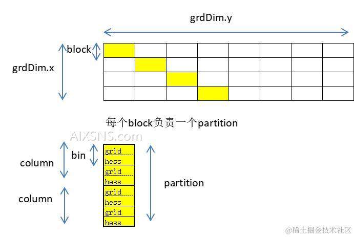
图1中上面的一张图展示了partition所对应的block在grid中的布局,下面的图展示单个block所负责的partition中数据布局:假如每个partition下有2个column,每个column分成2个bin,存储时每个bin下有2个位置,分别用于存储一个单元的gradients和hessians数据。
熟悉了参数的维度和数据布局之后,下面我们来详细介绍kernel中直方图的构建过程。kernel使用二维grid,x维度对应feature,y维度对应data,在x维度下每个block负责一个特征分区。x和y两个维度的线程总size(gridDim*blockDim)通常少于n_column和n_feature,所以grid下有的线程可能要负责多份数据,在代码的44~46行,67~79行两个循环体针对n_column_per_partition>blockDim.x和n_data_hat>gridDim.y*blockDim.y所做的兼容。同时n_feature和n_data_hat往往并不能恰好被blockDim和gridDim整除,代码56~61行也针对性做了兼容。
整个kernel运行执行分为3个步骤:
- 将global_hist_buffer存放数据地方的值初始化0;
- 根据数据索引从cuda_gradients, cuda_hessians获取对应数据的grad和hess值,累加到global_hist_buffer对应地址的bin上;
- 更新smaller_leaf_splits直方图属性值。
第41行shared_hist定位到了当前block负责的partition在global_hist_buffer中起始数据位置。然后第44~46行对该block负责分区中的hist数据初始化为0。第49到第64行定义了一些索引,并针对不能整除的场景做了相应的兼容。
第66行shared_hist_ptr定位到了当前partition下、当前column在global_hist_buffer中的grid和hess起始数据位置。67~79行为直方图构建的主体部分,首先根据smaller_leaf_splits下的data_indices_in_leaf找到叶子节点样本集在data中的索引,然后根据索引从cuda_gradients, cuda_hessians获取grad和hess值。第75行pos_ptr定位到了当前partition、当前column、当前bin在global_hist_buffer中起始数据位置,然后76,77行分别将获取的grid和hess值使用原子操作累加到global_hist_buffer对应的hist bin上。
最后在第84~87行对smaller_leaf_splits中属性hist_in_leaf的值进行更新,直方图构建完成。
直方图运算
直方图运算算子有2类,分别是直方图减法算子(SubtractHistogramKernel)和直方图“修剪”(FixHistogramKernel)。直方图减法算子非常简单,cuda_larger_leaf_splits直方图的grad和hess分别减去cuda_smaller_leaf_splits直方图的grad和hess:
// cuda_histogram_constructor.cu
__global__ void SubtractHistogramKernel(
        const int num_total_bin,
        const CUDALeafSplitsStruct* cuda_smaller_leaf_splits,
        const CUDALeafSplitsStruct* cuda_larger_leaf_splits) {
    const unsigned int global_thread_index = threadIdx.x + blockIdx.x * blockDim.x;
    const int cuda_larger_leaf_index = cuda_larger_leaf_splits->leaf_index;
    if (cuda_larger_leaf_index >= 0) {
        const hist_t* smaller_leaf_hist = cuda_smaller_leaf_splits->hist_in_leaf;
        hist_t* larger_leaf_hist = cuda_larger_leaf_splits->hist_in_leaf;
        if (global_thread_index < 2 * num_total_bin) {
            // larger_leaf_hist 的grad和hess分别减去smaller_leaf_hist的grad和hess
            larger_leaf_hist[global_thread_index] -= smaller_leaf_hist[global_thread_index];
        }
    }
}
直方图的“修剪”算子如下,其作用是找到cuda_smaller_leaf_splits中需要fix的feature,将该feature下频次最高的bin对应的grad和hess值修改为cuda_smaller_leaf_splits全局之和-该feature局部之和:
__global__ void FixHistogramKernel(
        const uint32_t* cuda_feature_num_bins,
        const uint32_t* cuda_feature_hist_offsets,
        const uint32_t* cuda_feature_most_freq_bins,
        const int* cuda_need_fix_histogram_features,
        const uint32_t* cuda_need_fix_histogram_features_num_bin_aligned,
        const CUDALeafSplitsStruct* cuda_smaller_leaf_splits) {

    // 定义一块共享内存,用于后续对该feature下各bin的grad和hess值规约求和
    __shared__ hist_t shared_mem_buffer[32];
    const unsigned int blockIdx_x = blockIdx.x;
    // 需要fix的feature索引
    const int feature_index = cuda_need_fix_histogram_features[blockIdx_x];
    // 需要fix的feature统一的bin个数
    const uint32_t num_bin_aligned = cuda_need_fix_histogram_features_num_bin_aligned[blockIdx_x];
    // 该feature对应直方图的offset
    const uint32_t feature_hist_offset = cuda_feature_hist_offsets[feature_index];
    // 该feature下频数最高的bin
    const uint32_t most_freq_bin = cuda_feature_most_freq_bins[feature_index];
    const double leaf_sum_gradients = cuda_smaller_leaf_splits->sum_of_gradients;
    const double leaf_sum_hessians = cuda_smaller_leaf_splits->sum_of_hessians;
    // 该feature直方图数据起始位置
    hist_t* feature_hist = cuda_smaller_leaf_splits->hist_in_leaf + feature_hist_offset * 2;
    const unsigned int threadIdx_x = threadIdx.x;
    // 该feature bin数量
    const uint32_t num_bin = cuda_feature_num_bins[feature_index];
    const uint32_t hist_pos = threadIdx_x << 1;
    const hist_t bin_gradient = (threadIdx_x < num_bin && threadIdx_x != most_freq_bin) ? feature_hist[hist_pos] : 0.0f;
    const hist_t bin_hessian = (threadIdx_x < num_bin && threadIdx_x != most_freq_bin) ? feature_hist[hist_pos + 1] : 0.0f;
    // 获取feature下各bin的grad和hess之和
    const hist_t sum_gradient = ShuffleReduceSum<hist_t>(bin_gradient, shared_mem_buffer, num_bin_aligned);
    const hist_t sum_hessian = ShuffleReduceSum<hist_t>(bin_hessian, shared_mem_buffer, num_bin_aligned);

    // 将频率最高bin下grad和hess值改为全局之和-该feature局部之和
    if (threadIdx_x == 0) {
        feature_hist[most_freq_bin << 1] = leaf_sum_gradients - sum_gradient;
        feature_hist[(most_freq_bin << 1) + 1] = leaf_sum_hessians - sum_hessian;
    }
}
其中参数cuda_need_fix_histogram_features存放了需要进行fix的feature,kernel使用的是1维的网格,每个block负责一个需要fix的feature,每个线程负责一个feature下的一个bin。FixHistogramKernel第23行定位到了线程负责的feature在hist_in_leaf的起始位置,然后第31行和32行分别计算了该feature下前num_bin_aligned个bin的局部grad、hess之和,第36、37行将全局之和减局部之和赋值该feature下most_freq_bin。
小结
以上我们介绍了LightGBM中直方图相关的cuda算子,包括直方图构建和直方图运算两类。直方图构建理解起来要稍微复杂一点。需要先了解数据的布局,特别是global_hist_buffer的scatter布局方式。后续我们将继续介绍boosting过程中其他业务类算子。
